Klausurvorbereitung

Libraries

library(MASS)
library(lmtest)
library(Ecdat)
library(sur)
library(plotly)
library(tidyverse)
library(gridExtra)

Einfache Regressionsmodelle

Regressions with Boston Housing Data

housing <- Boston
?Boston

housing %>% ggplot(aes(x=lstat, y=medv))+
  geom_point()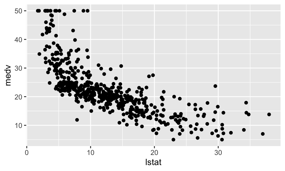

Regression Nummer 1 mit \(\text{medv} = \beta_1 + \beta_2 \cdot \text{lstat}\)

Reg1 <- lm(formula = medv ~ lstat+1, data = housing)
summary(Reg1)

Call:
lm(formula = medv ~ lstat + 1, data = housing)

Residuals:
    Min      1Q  Median      3Q     Max 
-15.168  -3.990  -1.318   2.034  24.500 

Coefficients:
            Estimate Std. Error t value Pr(>|t|)    
(Intercept) 34.55384    0.56263   61.41   <2e-16 ***
lstat       -0.95005    0.03873  -24.53   <2e-16 ***
---
Signif. codes:  0 '***' 0.001 '**' 0.01 '*' 0.05 '.' 0.1 ' ' 1

Residual standard error: 6.216 on 504 degrees of freedom
Multiple R-squared:  0.5441,    Adjusted R-squared:  0.5432 
F-statistic: 601.6 on 1 and 504 DF,  p-value: < 2.2e-16

housing %>% ggplot(aes(x=lstat, y=medv))+
  geom_point()+
  geom_abline(intercept = Reg1$coefficients[1], slope = Reg1$coefficients[2])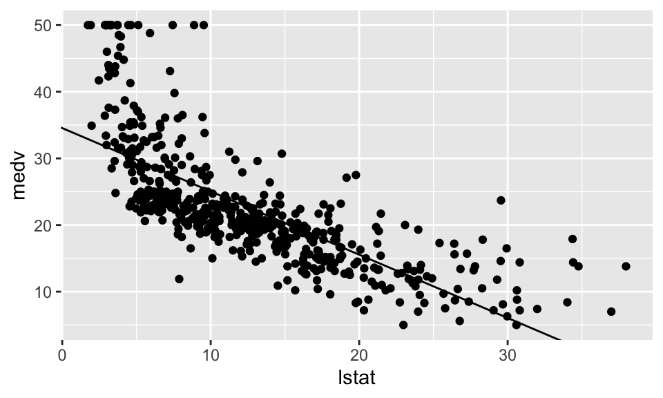

resettest(medv ~ lstat , power=2, type="regressor", data = housing)

    RESET test

data:  medv ~ lstat
RESET = 135.2, df1 = 1, df2 = 503, p-value < 2.2e-16

Regression Nummer 2 mit \(\ln(\text{medv}) = \beta_1 + \beta_2 \cdot \text{lstat}\)

Reg2 <- lm(formula = log(medv)~lstat, data = housing)
summary(Reg2)

Call:
lm(formula = log(medv) ~ lstat, data = housing)

Residuals:
     Min       1Q   Median       3Q      Max 
-0.94921 -0.14838 -0.02043  0.11441  0.90958 

Coefficients:
             Estimate Std. Error t value Pr(>|t|)    
(Intercept)  3.617572   0.021971  164.65   <2e-16 ***
lstat       -0.046080   0.001513  -30.46   <2e-16 ***
---
Signif. codes:  0 '***' 0.001 '**' 0.01 '*' 0.05 '.' 0.1 ' ' 1

Residual standard error: 0.2427 on 504 degrees of freedom
Multiple R-squared:  0.6481,    Adjusted R-squared:  0.6474 
F-statistic: 928.1 on 1 and 504 DF,  p-value: < 2.2e-16

housing %>% ggplot(aes(lstat, medv))+
  geom_point()+
  scale_y_continuous(trans = "log")+
  geom_abline(intercept = Reg2$coefficients[1], slope = Reg2$coefficients[2])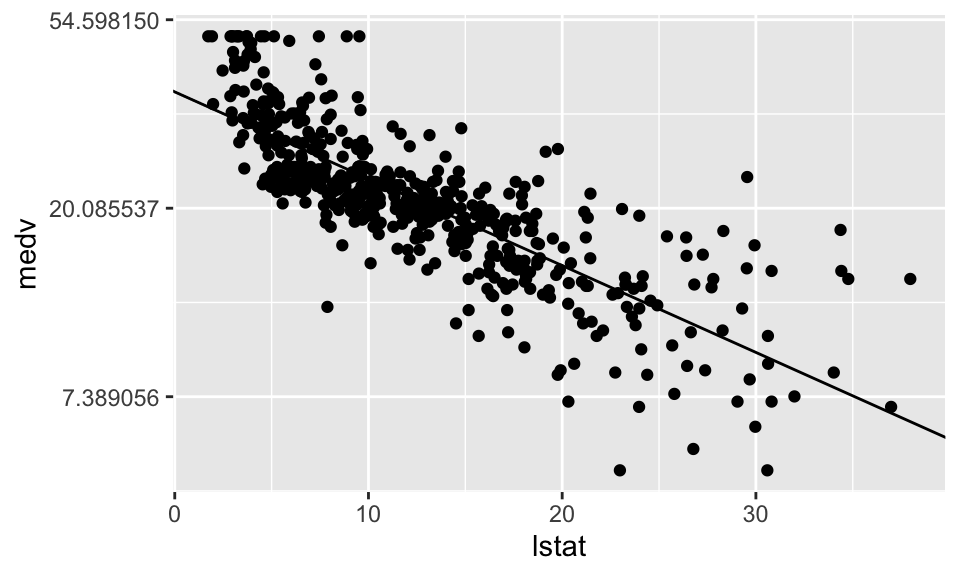

Regression Nummer 3 mit \(\ln(\text{medv}) = \beta_1 + \beta_2 \cdot \text{lstat} + \beta_3 \cdot \text{lstat}^2\)

Reg3 <- lm(formula = medv ~ lstat+I(lstat^2), data = housing)
summary(Reg3)

Call:
lm(formula = medv ~ lstat + I(lstat^2), data = housing)

Residuals:
     Min       1Q   Median       3Q      Max 
-15.2834  -3.8313  -0.5295   2.3095  25.4148 

Coefficients:
             Estimate Std. Error t value Pr(>|t|)    
(Intercept) 42.862007   0.872084   49.15   <2e-16 ***
lstat       -2.332821   0.123803  -18.84   <2e-16 ***
I(lstat^2)   0.043547   0.003745   11.63   <2e-16 ***
---
Signif. codes:  0 '***' 0.001 '**' 0.01 '*' 0.05 '.' 0.1 ' ' 1

Residual standard error: 5.524 on 503 degrees of freedom
Multiple R-squared:  0.6407,    Adjusted R-squared:  0.6393 
F-statistic: 448.5 on 2 and 503 DF,  p-value: < 2.2e-16

housing %>% ggplot(aes(x=lstat, y=medv))+
  geom_point()+
  stat_function(fun = function(x)
    {Reg3$coefficients[1] + Reg3$coefficients[2]*x + Reg3$coefficients[3]*x^2})

resettest(medv ~ lstat+I(lstat^2) , power=2, type="regressor", data = housing)

    RESET test

data:  medv ~ lstat + I(lstat^2)
RESET = 9.3452, df1 = 2, df2 = 501, p-value = 0.0001036

Regression Nummer 4 mit \(\ln(\text{medv}) = \beta_1 + \beta_2 \cdot \text{lstat} + \beta_3 \cdot \text{lstat}^2 + \beta_4 \cdot \text{lstat}^3\)

Reg4 <- lm(formula = medv ~ lstat+I(lstat^2)+I(lstat^3), data = housing)
summary(Reg4)

Call:
lm(formula = medv ~ lstat + I(lstat^2) + I(lstat^3), data = housing)

Residuals:
     Min       1Q   Median       3Q      Max 
-14.5441  -3.7122  -0.5145   2.4846  26.4153 

Coefficients:
              Estimate Std. Error t value Pr(>|t|)    
(Intercept) 48.6496253  1.4347240  33.909  < 2e-16 ***
lstat       -3.8655928  0.3287861 -11.757  < 2e-16 ***
I(lstat^2)   0.1487385  0.0212987   6.983 9.18e-12 ***
I(lstat^3)  -0.0020039  0.0003997  -5.013 7.43e-07 ***
---
Signif. codes:  0 '***' 0.001 '**' 0.01 '*' 0.05 '.' 0.1 ' ' 1

Residual standard error: 5.396 on 502 degrees of freedom
Multiple R-squared:  0.6578,    Adjusted R-squared:  0.6558 
F-statistic: 321.7 on 3 and 502 DF,  p-value: < 2.2e-16

housing %>% ggplot(aes(x=lstat, y=medv))+
  geom_point()+
  stat_function(fun = function(x)
  {Reg4$coefficients[1] + Reg4$coefficients[2]*x + Reg4$coefficients[3]*x^2 + Reg4$coefficients[4]*x^3})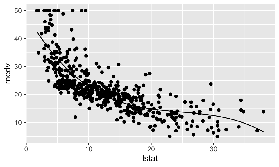

resettest(medv ~ lstat+I(lstat^2)+I(lstat^3) , power=2, type="regressor", data = housing)

    RESET test

data:  medv ~ lstat + I(lstat^2) + I(lstat^3)
RESET = 12.165, df1 = 3, df2 = 499, p-value = 1.076e-07

Prüfen auf Einflussreiche Beobachtungen und Außreißer

length(housing$medv)

[1] 506

column1 <- seq(1,1, length.out=506)
matrix <- cbind(column1, housing$lstat)

hatMatrix <- matrix %*% solve(t(matrix) %*% matrix) %*% t(matrix)
diagHatMatrix <- diag(hatMatrix)

show(diagHatMatrix)

  [1] 0.004262518 0.002455527 0.004863680 0.005639779 0.004058706 0.004127513
  [7] 0.001978217 0.003615365 0.013567169 0.002744185 0.004336932 0.001991064
 [13] 0.002339159 0.002725692 0.002198662 0.002655757 0.003408468 0.002134252
 [19] 0.002012300 0.002049494 0.004694701 0.002030073 0.003405580 0.004004395
 [25] 0.002492748 0.002553939 0.002156943 0.002807608 0.001977123 0.001993876
 [31] 0.005818324 0.001982098 0.010779804 0.003236561 0.004270793 0.002319519
 [37] 0.002036287 0.002561791 0.002223479 0.004672735 0.006399736 0.004346707
 [43] 0.003794663 0.003031568 0.002350192 0.002208052 0.002063299 0.003443523
 [49] 0.014778002 0.002464813 0.002000947 0.002379670 0.004087240 0.002668814
 [55] 0.002155272 0.004364946 0.003815983 0.004917504 0.003279450 0.002433949
 [61] 0.001985874 0.002100279 0.003338594 0.002362339 0.002799052 0.004450983
 [67] 0.002202395 0.002781274 0.001983698 0.002555776 0.003343198 0.002274893
 [73] 0.003952049 0.002991470 0.003315691 0.002511647 0.001994402 0.002196808
 [79] 0.001980090 0.002466502 0.004081517 0.003122517 0.003343198 0.003003418
 [85] 0.002333513 0.003432148 0.001977947 0.002665538 0.003963144 0.003853592
 [91] 0.002549791 0.002746302 0.002760198 0.003588295 0.002141560 0.003375643
 [97] 0.002043235 0.004744393 0.005179954 0.003598318 0.002382178 0.002940504
[103] 0.002135213 0.002000332 0.001980337 0.002542020 0.003377449 0.002056463
[109] 0.001981983 0.002302167 0.001980959 0.002217636 0.002467572 0.002740735
[115] 0.002164752 0.002351126 0.001990879 0.002191290 0.002262928 0.002011844
[121] 0.002090755 0.002077809 0.003057586 0.008295685 0.002918905 0.002156943
[127] 0.010261454 0.002775582 0.002267164 0.003232141 0.001976394 0.001982284
[133] 0.002067549 0.002195675 0.002818424 0.002696596 0.002676666 0.002121969
[139] 0.004893136 0.003285699 0.007117935 0.020357684 0.009769828 0.009335944
[145] 0.012724338 0.010885361 0.002596636 0.013036672 0.011507565 0.004981295
[151] 0.002057583 0.001991547 0.001987319 0.002358400 0.002212604 0.002193833
[157] 0.002448425 0.004500830 0.003480090 0.003051908 0.003963144 0.006609388
[163] 0.006449610 0.005358735 0.002016137 0.002290159 0.005088907 0.001986506
[169] 0.002069946 0.002045290 0.002098895 0.001991359 0.002137400 0.002483198
[175] 0.002328817 0.004058706 0.002227414 0.003548513 0.003252596 0.004226903
[181] 0.002983544 0.002374680 0.004358858 0.003864408 0.002044657 0.001985874
[187] 0.004589259 0.003361691 0.004519651 0.004024722 0.004191568 0.004438598
[193] 0.005692773 0.004232820 0.004634045 0.005617183 0.004830292 0.002611037
[199] 0.003389664 0.004519651 0.004589259 0.003035620 0.005512663 0.005012891
[205] 0.005685179 0.002099742 0.002086282 0.003111519 0.002132690 0.006206176
[211] 0.002804019 0.006958334 0.002419106 0.002392283 0.013062901 0.002369720
[217] 0.002004800 0.002317214 0.003053492 0.002156295 0.002312627 0.004988131
[223] 0.002264222 0.002967784 0.004790484 0.004475844 0.005497855 0.003514111
[229] 0.004937816 0.005047327 0.002015354 0.004104453 0.006002898 0.004917504
[235] 0.002799052 0.002098361 0.002352606 0.004413923 0.003514111 0.003060098
[241] 0.002039218 0.001978771 0.002056031 0.004139089 0.001977194 0.003285699
[247] 0.002450086 0.002219576 0.002357457 0.003417917 0.003747147 0.005165862
[253] 0.005208233 0.005201152 0.003413189 0.002425985 0.005512663 0.004179852
[259] 0.002894623 0.003261516 0.002340615 0.003105701 0.003741906 0.002052728
[265] 0.002781274 0.002164752 0.002153608 0.003031568 0.005475703 0.002014878
[271] 0.001980959 0.003403756 0.002917424 0.003408468 0.005208233 0.005609667
[277] 0.003669351 0.004777276 0.003135210 0.004340643 0.005047327 0.004500830
[283] 0.005587165 0.005475703 0.002872102 0.002735962 0.001979263 0.003156521
[289] 0.002967784 0.002359894 0.005351491 0.005187012 0.004432418 0.002620491
[295] 0.002173404 0.003558412 0.003051908 0.002370678 0.004268481 0.004407774
[301] 0.003659110 0.002362339 0.002592337 0.004334587 0.003248147 0.002514534
[307] 0.003460820 0.002995445 0.004532237 0.002255825 0.001976291 0.003705438
[313] 0.002010091 0.002853548 0.002418091 0.002027913 0.003227728 0.002395817
[319] 0.002180465 0.001976514 0.003130971 0.003274955 0.002928929 0.002008658
[325] 0.003633644 0.004203315 0.003618458 0.001977013 0.002255825 0.003072442
[331] 0.002469266 0.001978217 0.002879578 0.003864408 0.003329410 0.002813413
[337] 0.002292371 0.002146402 0.002642825 0.002305805 0.002415475 0.003968703
[343] 0.002598539 0.003139457 0.004488322 0.002151313 0.001976296 0.003514111
[349] 0.003700260 0.003752395 0.003705438 0.003968703 0.002894623 0.004557503
[355] 0.002799052 0.003924448 0.002926574 0.001991064 0.002029720 0.001976296
[361] 0.002894623 0.002068011 0.002211862 0.002129588 0.004081517 0.003165100
[367] 0.002046734 0.001994079 0.005402365 0.005068082 0.005624707 0.002355028
[373] 0.002529089 0.020971010 0.026865167 0.002000332 0.006328634 0.004839537
[379] 0.006706492 0.005210978 0.002782645 0.004733829 0.006629662 0.007481612
[385] 0.014525439 0.014778002 0.011458958 0.016496011 0.014511481 0.004585358
[391] 0.002747643 0.003424489 0.008566016 0.002222280 0.002507007 0.002751108
[397] 0.003728250 0.004026908 0.014469655 0.013620902 0.009714913 0.004258869
[403] 0.004252918 0.003943126 0.010398143 0.006117484 0.006411243 0.001986909
[409] 0.009314576 0.003948657 0.002227414 0.004826215 0.020290158 0.004118201
[415] 0.024956703 0.012416477 0.008677773 0.009573043 0.004440995 0.005927236
[421] 0.002193833 0.002336788 0.002057583 0.006369841 0.002765047 0.007325531
[427] 0.002334426 0.002111630 0.005029309 0.007046690 0.002942004 0.003899157
[433] 0.001991359 0.002470338 0.002222280 0.006353335 0.003107324 0.009368054
[439] 0.019704605 0.006037670 0.005449119 0.003807372 0.002578151 0.003467489
[445] 0.006792596 0.006958334 0.003000972 0.002533161 0.003141104 0.003697091
[451] 0.002866097 0.002977175 0.002804019 0.002624888 0.003400872 0.003141104
[457] 0.003545487 0.002689921 0.002473112 0.002138986 0.002527295 0.002131135
[463] 0.002045692 0.002193122 0.001988766 0.002060989 0.002761550 0.004893136
[469] 0.003141104 0.002148664 0.002489920 0.001978112 0.002089425 0.002014579
[475] 0.003145361 0.007064455 0.003386795 0.007810023 0.003098957 0.001984392
[481] 0.002118400 0.002913604 0.003212838 0.002169920 0.001994608 0.002143166
[487] 0.002186542 0.002032488 0.003111519 0.006949541 0.013234152 0.003115722
[493] 0.001995146 0.001992343 0.002010373 0.002926574 0.004773237 0.002057583
[499] 0.001979052 0.002208788 0.002085483 0.002321832 0.002472037 0.003886132
[505] 0.003456022 0.002860947

# jetzt müsste geprüft werden welche Zeilen der diagHatMatrix größer sind als 2*(2/506)

as.data.frame(diagHatMatrix) %>%
  mutate(n = 1:nrow(.)) %>%
  filter(diagHatMatrix > 2*(2/506))

Auf Koliniarität prüfen

Reg5 <- lm(formula = log(medv) ~ lstat + crim, data = housing)
summary(Reg5)

Call:
lm(formula = log(medv) ~ lstat + crim, data = housing)

Residuals:
     Min       1Q   Median       3Q      Max 
-0.78707 -0.15045 -0.02918  0.11439  0.88271 

Coefficients:
             Estimate Std. Error t value Pr(>|t|)    
(Intercept)  3.585383   0.021417 167.409  < 2e-16 ***
lstat       -0.040776   0.001620 -25.175  < 2e-16 ***
crim        -0.009665   0.001345  -7.187  2.4e-12 ***
---
Signif. codes:  0 '***' 0.001 '**' 0.01 '*' 0.05 '.' 0.1 ' ' 1

Residual standard error: 0.2314 on 503 degrees of freedom
Multiple R-squared:  0.6809,    Adjusted R-squared:  0.6796 
F-statistic: 536.5 on 2 and 503 DF,  p-value: < 2.2e-16

plot_ly(x=housing$lstat, y=housing$crim, z=log(housing$medv), 
        type="scatter3d", mode="markers", color=housing$lstat, size=15)

Ein paar Tests

Einfache Regression

n <- 40
quadratmeter <- seq(n)
preis <- rnorm(n,0+3*quadratmeter, 40)
data <- data.frame(quadratmeter, preis)

a1 <- lm(preis~quadratmeter)
summary(a1)

Call:
lm(formula = preis ~ quadratmeter)

Residuals:
    Min      1Q  Median      3Q     Max 
-82.762 -34.350   3.379  32.215  70.983 

Coefficients:
             Estimate Std. Error t value Pr(>|t|)   
(Intercept)   24.5103    13.1134   1.869  0.06933 . 
quadratmeter   1.8730     0.5574   3.360  0.00178 **
---
Signif. codes:  0 '***' 0.001 '**' 0.01 '*' 0.05 '.' 0.1 ' ' 1

Residual standard error: 40.69 on 38 degrees of freedom
Multiple R-squared:  0.2291,    Adjusted R-squared:  0.2088 
F-statistic: 11.29 on 1 and 38 DF,  p-value: 0.001783

data %>% ggplot(aes(quadratmeter, preis))+
  geom_point()+
  stat_function(fun = function(x)  {a1$coefficients[1] + a1$coefficients[2]*x})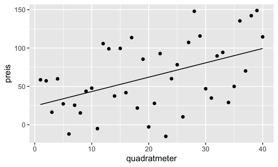

Heteroskedastizität

Generierung von Heteroskedastizität und Verteilung der Residuen

n2 <- 10000
x <- runif(n2, min = 0, max = 10)
y <- rnorm(n2, mean = 50+3*x, sd = 5+2*x)
df1 <- data.frame(x, y)
df1 %>%
  ggplot(aes(x, y))+
  geom_point(alpha = .5, size = .5)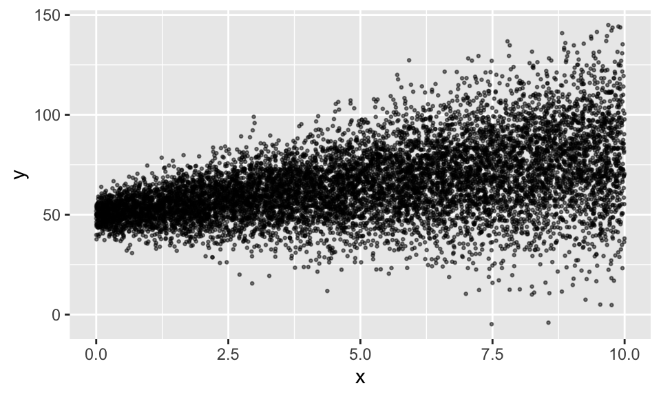

a2 <- lm(y~x)
summary(a2)

Call:
lm(formula = y ~ x)

Residuals:
    Min      1Q  Median      3Q     Max 
-79.653  -9.003   0.068   8.915  65.926 

Coefficients:
            Estimate Std. Error t value Pr(>|t|)    
(Intercept) 49.91845    0.32474  153.72   <2e-16 ***
x            2.99971    0.05626   53.32   <2e-16 ***
---
Signif. codes:  0 '***' 0.001 '**' 0.01 '*' 0.05 '.' 0.1 ' ' 1

Residual standard error: 16.15 on 9998 degrees of freedom
Multiple R-squared:  0.2214,    Adjusted R-squared:  0.2213 
F-statistic:  2843 on 1 and 9998 DF,  p-value: < 2.2e-16

a2 %>% ggplot(aes(x=a2$residuals))+
  geom_density()+
  stat_function(fun = function(x){dnorm(x, mean = mean(a2$residuals), sd = sd(a2$residuals))}, linetype = "dashed")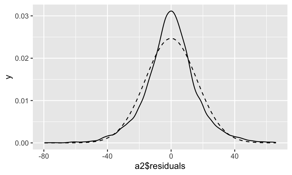

Die Residuen (durchgezogene Linie) sind nicht normalverteilt (gestrichelte Linie)

Beispiel einer fehlehnden Binärvariable

n <- 500
data <- data.frame(x = runif(n, min = 0, max = 10),
           group = c(1,2)) %>%
  mutate(group = as.factor(group),
         y = if_else(group == 1, 
                     5 + 3*x + rnorm(n, 0, 2), 
                     20 + 3*x + rnorm(n, 0, 2)))

data %>%
  ggplot(aes(x = x, y = y, color = group))+
  geom_point()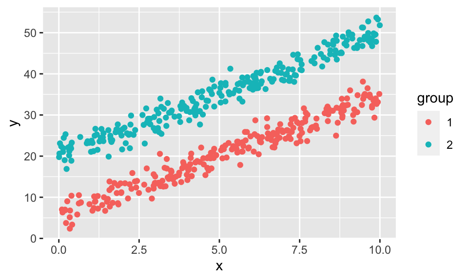

reg1 <- lm(y ~ x, data = data)
reg1

Call:
lm(formula = y ~ x, data = data)

Coefficients:
(Intercept)            x  
     13.315        2.846  

data.frame(resid = resid(reg1)) %>%
  ggplot(aes(x = resid))+
  geom_histogram(bins = 30)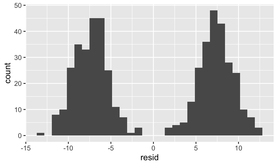

reg2 <- lm(y ~ x + group, data = data)
reg2

Call:
lm(formula = y ~ x + group, data = data)

Coefficients:
(Intercept)            x       group2  
      5.326        2.957       14.839  

data.frame(resid = resid(reg2)) %>%
  ggplot(aes(x = resid))+
  geom_histogram(bins = 30)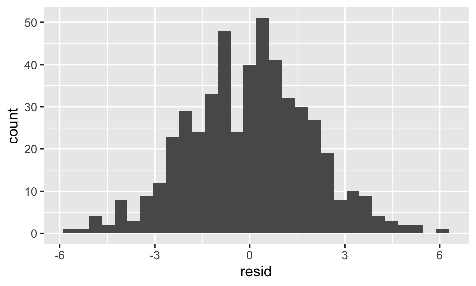

Chow Test für Strukturbruch

Wir generieren zuerst einen Datensatz mit einem Strukturbruch bei \(x=0\). Es soll nicht zu offensichtlich sein, damit der F-Test am Ende noch interessant bleibt.

n <- 200

x1 <- runif(n/2, min = -5, max = 0)
x2 <- runif(n/2, min = 0, max = 5)

y1 <- 5 + 1*x1 + rnorm(n/2, 0, 3)
y2 <- 5 + 3*x2 + rnorm(n/2, 0, 3)

data <- data.frame(x = c(x1, x2), y = c(y1, y2))

data %>%
  ggplot(aes(x, y))+
  geom_point()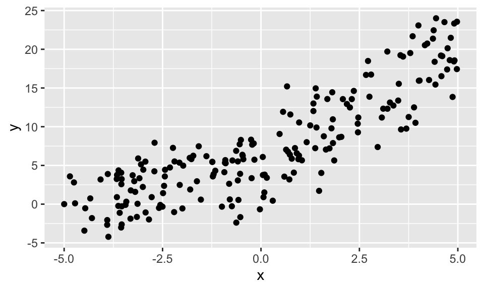

Wir sehen, dass eine “naive” lineare Regression hier kein gutes Ergebnis bringt.

reg1 <- lm(y ~ x, data = data)
summary(reg1)

Call:
lm(formula = y ~ x, data = data)

Residuals:
    Min      1Q  Median      3Q     Max 
-8.6773 -2.4415 -0.0878  2.4663  7.4319 

Coefficients:
            Estimate Std. Error t value Pr(>|t|)    
(Intercept)  7.32257    0.24542   29.84   <2e-16 ***
x            2.08198    0.08697   23.94   <2e-16 ***
---
Signif. codes:  0 '***' 0.001 '**' 0.01 '*' 0.05 '.' 0.1 ' ' 1

Residual standard error: 3.468 on 198 degrees of freedom
Multiple R-squared:  0.7432,    Adjusted R-squared:  0.7419 
F-statistic: 573.1 on 1 and 198 DF,  p-value: < 2.2e-16

data %>% ggplot(aes(x, y))+
  geom_point()+
  geom_abline(intercept = reg1$coefficients[1], slope = reg1$coefficients[2])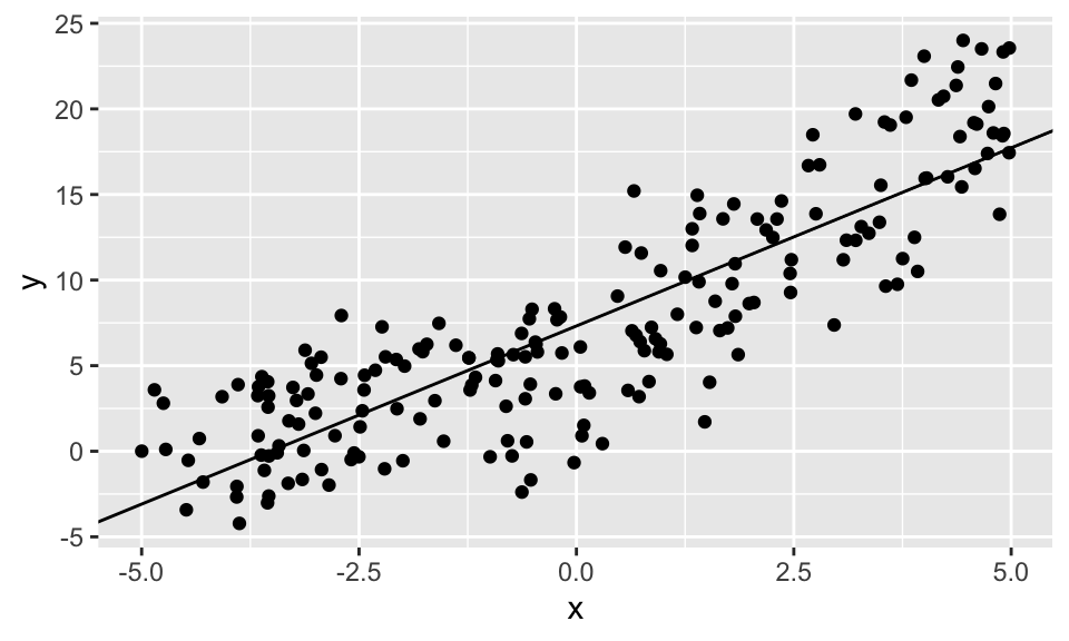

reg2.1 <- lm(y ~ x, data = data %>% filter(x < 0))
reg2.2 <- lm(y ~ x, data = data %>% filter(x > 0))

data %>% ggplot(aes(x, y))+
  geom_point()+
  geom_abline(intercept = reg2.1$coefficients[1], slope = reg2.1$coefficients[2])+
  geom_abline(intercept = reg2.2$coefficients[1], slope = reg2.2$coefficients[2])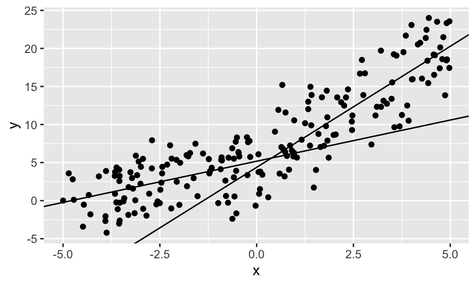

Der Chow Test zeigt ganz klar, dass ein Strukturbruch vorliegt.

SSR.R <- sum(resid(reg1)^2)
SSR.U <- sum(resid(reg2.1)^2) + sum(resid(reg2.2)^2)

Fstatistic <- ((SSR.R-SSR.U)/reg1$rank)/(SSR.U/(n - 2*reg1$rank))
Fstatistic

[1] 24.32638

1-pf(Fstatistic, reg1$rank, n - 2*reg1$rank)

[1] 3.657481e-10

Echte Daten

Aus den Übungen

data("Bwages")
d <- Bwages
?Bwages
#d

data("Caschool")
#Caschool
?Caschool

data("Icecream")
#Icecream
?Icecream

Reg1 <- lm(formula = cons~price+temp+I(price*temp), data = Icecream)
summary(Reg1)

Call:
lm(formula = cons ~ price + temp + I(price * temp), data = Icecream)

Residuals:
      Min        1Q    Median        3Q       Max 
-0.093826 -0.021935  0.006617  0.020962  0.082094 

Coefficients:
                Estimate Std. Error t value Pr(>|t|)
(Intercept)     -0.17029    0.89149  -0.191    0.850
price            1.38220    3.23280   0.428    0.672
temp             0.01880    0.01755   1.071    0.294
I(price * temp) -0.05731    0.06375  -0.899    0.377

Residual standard error: 0.04146 on 26 degrees of freedom
Multiple R-squared:  0.6439,    Adjusted R-squared:  0.6028 
F-statistic: 15.67 on 3 and 26 DF,  p-value: 5.07e-06

plot(Icecream$price ,Icecream$cons)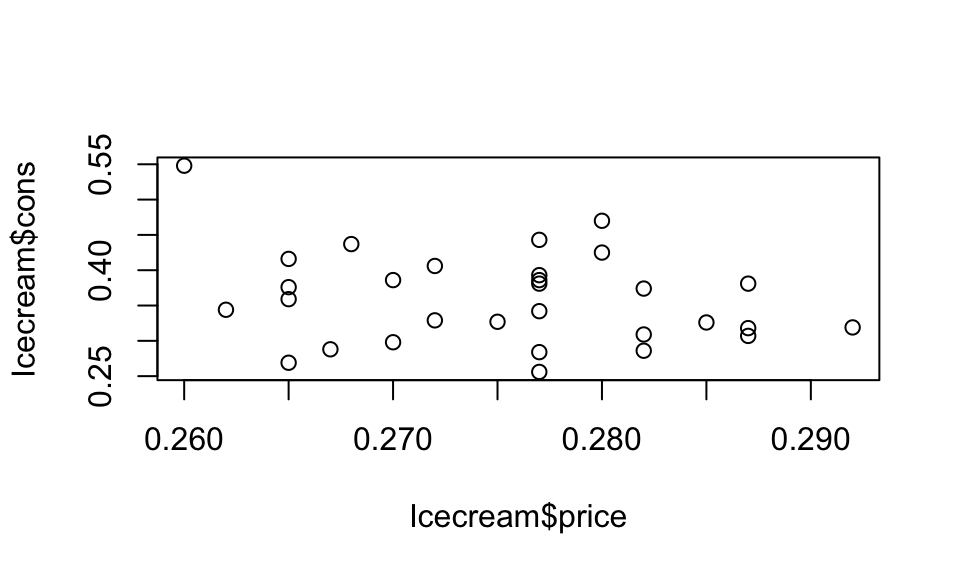

Reg2 <- lm(formula = cons~temp, data = Icecream)
summary(Reg2)

Call:
lm(formula = cons ~ temp, data = Icecream)

Residuals:
      Min        1Q    Median        3Q       Max 
-0.069411 -0.024478 -0.007371  0.029126  0.120516 

Coefficients:
             Estimate Std. Error t value Pr(>|t|)    
(Intercept) 0.2068621  0.0247002   8.375 4.13e-09 ***
temp        0.0031074  0.0004779   6.502 4.79e-07 ***
---
Signif. codes:  0 '***' 0.001 '**' 0.01 '*' 0.05 '.' 0.1 ' ' 1

Residual standard error: 0.04226 on 28 degrees of freedom
Multiple R-squared:  0.6016,    Adjusted R-squared:  0.5874 
F-statistic: 42.28 on 1 and 28 DF,  p-value: 4.789e-07

Reg2.1 <- lm(testscr~I(expnstu/1000)+compstu, data = Caschool)
summary(Reg2.1)

Call:
lm(formula = testscr ~ I(expnstu/1000) + compstu, data = Caschool)

Residuals:
    Min      1Q  Median      3Q     Max 
-52.815 -13.787  -0.116  13.078  47.016 

Coefficients:
                Estimate Std. Error t value Pr(>|t|)    
(Intercept)      625.000      7.528  83.024  < 2e-16 ***
I(expnstu/1000)    3.723      1.468   2.537   0.0116 *  
compstu           68.993     14.323   4.817 2.04e-06 ***
---
Signif. codes:  0 '***' 0.001 '**' 0.01 '*' 0.05 '.' 0.1 ' ' 1

Residual standard error: 18.25 on 417 degrees of freedom
Multiple R-squared:  0.08736,   Adjusted R-squared:  0.08299 
F-statistic: 19.96 on 2 and 417 DF,  p-value: 5.272e-09

Reg2.2 <- lm(testscr~I(expnstu/1000), data = Caschool)
summary(Reg2.2)

Call:
lm(formula = testscr ~ I(expnstu/1000), data = Caschool)

Residuals:
    Min      1Q  Median      3Q     Max 
-50.146 -14.206   0.689  13.513  50.127 

Coefficients:
                Estimate Std. Error t value Pr(>|t|)    
(Intercept)      623.617      7.720  80.783  < 2e-16 ***
I(expnstu/1000)    5.749      1.443   3.984 7.99e-05 ***
---
Signif. codes:  0 '***' 0.001 '**' 0.01 '*' 0.05 '.' 0.1 ' ' 1

Residual standard error: 18.72 on 418 degrees of freedom
Multiple R-squared:  0.03659,   Adjusted R-squared:  0.03428 
F-statistic: 15.87 on 1 and 418 DF,  p-value: 7.989e-05

Sterbedaten Deutschland

Quelle: Genesis Tabelle 12613-0003

data <- read_csv2("/Users/sebastiangeis/Downloads/12613-0003_$F_flat (1).csv") %>%
  janitor::clean_names() %>%
  select(jahr = zeit, geschlecht = x2_auspraegung_code, alter = x3_auspraegung_code, anzahl = bev002_gestorbene_anzahl) %>%
  mutate(geschlecht = str_extract(geschlecht, ".{1}$") %>% factor(),
         alter = str_extract(alter, "\\d{3}$") %>% as.numeric(),
         anzahl = as.numeric(anzahl)) %>%
  drop_na()
head(data)

data_uncounted <- data %>%
  uncount(anzahl)
head(data_uncounted)

Der originale Datensatz gibt die Anzahl an Toten je Jahr, Alter und Geschlecht an. Wir transformieren den Datensatz, damit jede Zeile einer Person entspricht. Diese Datensatz hat dann 60356559 Zeilen. Das ist sehr viel, daher verwenden wir für die Regressionen jeweils nur eine Stichprobe.

data_uncounted %>%
  group_by(jahr, geschlecht) %>%
  summarise(alter = mean(alter)) %>%
  ggplot(aes(x = jahr, y = alter, color = geschlecht))+
  geom_line()

`summarise()` has grouped output by 'jahr'. You can override using the
`.groups` argument.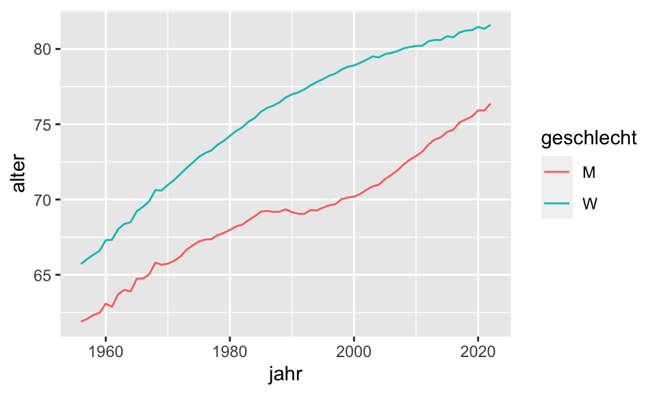

reg1 <- lm(alter ~ jahr, data = data_uncounted %>% slice_sample(n = 100000))
summary(reg1)

Call:
lm(formula = alter ~ jahr, data = data_uncounted %>% slice_sample(n = 1e+05))

Residuals:
    Min      1Q  Median      3Q     Max 
-79.582  -6.217   3.708  10.867  32.746 

Coefficients:
              Estimate Std. Error t value Pr(>|t|)    
(Intercept) -3.551e+02  5.380e+00  -66.00   <2e-16 ***
jahr         2.150e-01  2.705e-03   79.48   <2e-16 ***
---
Signif. codes:  0 '***' 0.001 '**' 0.01 '*' 0.05 '.' 0.1 ' ' 1

Residual standard error: 16.56 on 99998 degrees of freedom
Multiple R-squared:  0.05941,   Adjusted R-squared:  0.0594 
F-statistic:  6317 on 1 and 99998 DF,  p-value: < 2.2e-16

reg2 <- lm(alter ~ jahr + geschlecht, data = data_uncounted %>% slice_sample(n = 100000))
summary(reg2)

Call:
lm(formula = alter ~ jahr + geschlecht, data = data_uncounted %>% 
    slice_sample(n = 1e+05))

Residuals:
    Min      1Q  Median      3Q     Max 
-82.604  -5.804   3.553  10.368  34.847 

Coefficients:
              Estimate Std. Error t value Pr(>|t|)    
(Intercept) -3.531e+02  5.293e+00  -66.71   <2e-16 ***
jahr         2.123e-01  2.661e-03   79.78   <2e-16 ***
geschlechtW  6.439e+00  1.031e-01   62.48   <2e-16 ***
---
Signif. codes:  0 '***' 0.001 '**' 0.01 '*' 0.05 '.' 0.1 ' ' 1

Residual standard error: 16.29 on 99997 degrees of freedom
Multiple R-squared:  0.09372,   Adjusted R-squared:  0.0937 
F-statistic:  5170 on 2 and 99997 DF,  p-value: < 2.2e-16

data.frame(reg1 = reg1$residuals, reg2 = reg2$residuals) %>%
  pivot_longer(cols = everything(), names_to = "model", values_to = "residuals") %>%
  ggplot(aes(x = residuals, color = model))+
  geom_density()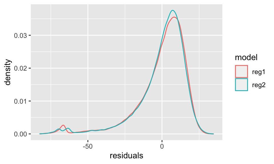

Betrachten wir den Plot mit dem durchschnittlichen Sterbealter, wird sofort klar, dass eine Binärvariable für das Geschlecht genutzt werden muss. In der Regression sehen wir dann, dass Frauen im Schnitt 6,6 Jahre länger leben als Männer.

Allerdings ist der Unterschied im Residuenplot nicht eindeutig. Für Regression 1, also ohne Berücksichtigung des Geschlechts, hätten wir zwei “Gipfel” erwartet. Dies ist nicht der Fall. Außerdem müssen wir die Verteilungsannahme überdenken, da die Residuen offensichtlich nicht normalverteilt sint. Hieran ändert auch eine log-Transofrmation nichts (nicht dargestellt).